Python(Visualise)--matplotlib

Matplotlib 是一个Python 2D绘图库，它可以在各种平台上以各种硬拷贝格式和交互式环境生成出具有出版品质的图形。 Matplotlib可用于Python脚本，Python和IPython shell，Jupyter笔记本，Web应用程序服务器和四个图形用户界面工具包

Pyplot

matplotlib.pyplot是matplotlib的基于状态的接口。它提供了类似MATLAB的绘图方式。

import matploblib.pyplot as plt

Workflow

• Step 1 Prepare data
• Step 2 Create figure
• Step 3 Add axes
• Step 4 Customize plot
• Step 5 Save plot
• Step 6 Show plot

>>> import matplotlib.pyplot as plt 
>>> x = [1,2,3,4] 
>>> y = [10,20,25,30] 
>>> fig = plt.figure() 
>>> ax = fig.add_subplot(111) 
>>> ax.plot(x, y, color='lightblue', linewidth=3)
>>> ax.set_xlim(1, 6.5) 
>>> plt.savefig('foo.png') 
>>> plt.show()

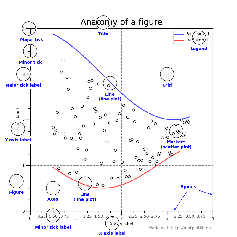
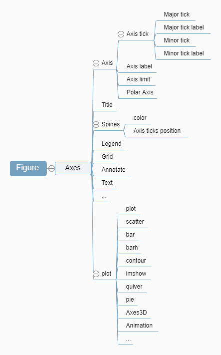
Figure and Axes

一般通过get_<part>方法获得组件属性，set_<part>方法重设组件。

Create Figure

plt.figure(num=None, figsize=None, dpi=None, facecolor=None, edgecolor,...)

Parameters:
num : (integer or string) figure编号
figsize : (tuple of integers) figure尺寸
dpi : (integer) 分辨率

Add Axes

fig.add_subplot(nrows, ncols, plot_number)

fig=plt.figure()
fig.add_subplot(221) # row-col-num

nrows, ncols, plot_number: 分割figure行数和列数，axes的位置

fig.add_axes(rect) 可以添加图中图

Parameters:
rect : [left, bottom, width, height]
projection : [‘aitoff’ | ‘hammer’ | ‘lambert’ | ‘mollweide’ | ‘polar’ | ‘rectilinear’], optional
polar : boolean, optional

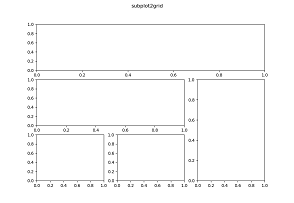
plt.subplot2grid(shape, loc, rowspan=1, colspan=1) 建造不规则axes

Parameters:
shape: figue分割
loc: 原点位置，基于shape分割结果
rowspan, colspan: 行或列的跨度

ax1 = plt.subplot2grid((3,3), (0,0), colspan=3)  
ax2 = plt.subplot2grid((3,3), (1,0), colspan=2)  
ax3 = plt.subplot2grid((3,3), (1, 2), rowspan=2)  
ax4 = plt.subplot2grid((3,3), (2, 0))  
ax5 = plt.subplot2grid((3,3), (2, 1))  
plt.suptitle("subplot2grid")  

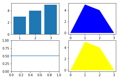
plt.subplots
plt.subplots(nrows=1, ncols=1, sharex=False, sharey=False,...) Create a figure and a set of subplots

Parameters:
nrows, ncols : (int) 分割figure行数和列数
sharex, sharey : bool or {‘none’, ‘all’, ‘row’, ‘col’}, 是否共享坐标轴

fig, ax = plt.subplots(2,2) 
f, (ax1, ax2) = plt.subplots(1, 2, sharey=True)

Plot

常用图形	说明
plot(x,y,data)	默认折线图
scatter(x, y, s, c, marker, cmap)	散点图{s:size,c:color}
hist(x, bins)	直方图
bar(x, height, width, fill)	柱状图
barh(y, height, width, fill)	横向柱状图
boxplot(y)	箱线图
violinplot(y)	小提琴
axhline(y)	水平线
axvline(x)	垂直线
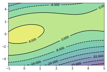
contourf(X,Y,Z,N,cmap)	等高线填充
contour(X,Y,Z,N)	等高线线条
imshow()	热图
quiver()	2D箭头场
streamplot()	2D矢量场
pie(x, explode, labels, colors)	饼图
acorr(x)	自相关
fill(x,y)	填充多边形
fill_between(x,y)	两曲线间填充

Parameters:
Alpha
Colors©, Color Bars & Color Maps(cmap)
Markers: marker , size
Line: linestyle(ls), linewidth

x=[0,1,2,3]
y=[0,5,4,0]
fig, axes = plt.subplots(2,2) 
axes[0,0].bar([1,2,3],[3,4,5])
axes[1,0].axhline(0.5)
axes[0,1].fill(x,y,color='blue')
axes[1,1].fill_between(x,y,color='yellow')

import numpy as np
import matplotlib.pyplot as plt

x=np.linspace(-1,5,500)
y=np.linspace(-5,5,500)
X,Y=np.meshgrid(x, y)
Height=10*np.sin(X)/X-Y**2+X*Y


plt.contourf(X, Y, Height,8, alpha = 0.6) # 填充颜色
C = plt.contour(X, Y, Height, 8,colors = 'black') # 绘制等高线
plt.clabel(C, inline = True, fontsize = 10) # 显示各等高线的数据标签
plt.show()

Parts of Axes

Axis(x axis)	说明
ax.set_xlabel(xlabel, fontdict=None, labelpad=None)	x轴标签
ax.set_xticks(ticks, minor=False)	x轴刻度
ax.set_xticklabels(labels, fontdict=None, minor=False)	x轴刻度标签
ax.set_xlim(left=None, right=None)	x轴限制
ax.axis(‘scaled’)	xy轴标准
ax.set_title(label, fontdict=None, loc=‘center’)	loc : {‘center’, ‘left’, ‘right’}, str, optional

# x轴刻度标签属性设置，其他组件属性设置基本相同
xlabel=ax.get_xticklabels()
label.set_fontsize(...)
label.set_bbox(...)

Spines

ax.spines['left'].set_color('b') # 左侧线条修改为蓝色
ax.spines['top'].set_visible(False) # 使顶层线条不可见
ax.spines['bottom'].set_position(('outward',10) # 使底层线条外移10

spines: {left,right,top,bottom}

Legend
ax.legend(loc='best', handles,labels)

handles:图例控制对象
labels:图例标签
loc: string or 0:10

Grid
ax.grid(b=None, which='major', axis='both')

Parameters:
which: ‘major’ (default), ‘minor’, or ‘both’
axis: ‘both’ (default), ‘x’, or ‘y’

annotate and Text

ax.annotate()

Parameters:
s : str
xy : iterable
xytext : iterable, optional
xycoords : str, Artist, Transform, callable or tuple, optional
textcoords : str, Artist, Transform, callable or tuple, optional
fontsize:
arrowprops : dict, optional

ax.text(x, y, s, fontdict=None, withdash=False)

Save and Show

fig.savefig(fname) # or plt.savefig
fig.show(warn=True) # or plt.show

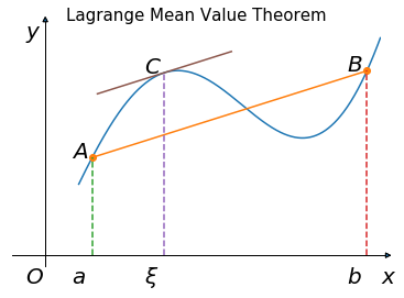
example

# ---------------------拉格朗日中值定理
import numpy as np
import matplotlib.pyplot as plt
from scipy.optimize import fsolve
import mpl_toolkits.axisartist as axisartist

xlim=(0.5,5)
x = np.linspace(xlim[0],xlim[1], 500)

def f(x):
    return x**2+10*np.sin(x)
def df(x,const): #导数方程
    return 2*x+10*np.cos(x)-const

a,b=0.7,4.8
slope=(f(b)-f(a))/(b-a) #AB斜率
c=fsolve(df,1,args=slope) #解非线性方程

def y(x):#切线方程y-y0=k(x-x0)
    return slope*(x-c)+f(c)

#添加画布
fig = plt.figure()
ax = axisartist.Subplot(fig, 111)#引入坐标轴对象
fig.add_axes(ax)#添加坐标轴
ax.axis[:].set_visible(False)#隐藏原坐标

#添加箭头坐标
ax.axis["x"] = ax.new_floating_axis(0,0)
ax.axis["x"].set_axisline_style("-|>",size = 1)
ax.axis["y"] = ax.new_floating_axis(1,0)
ax.axis["y"].set_axisline_style("-|>", size = 1)

#添加xOy标签
ax.axis('scaled')
ax.set_xlim(-0.5,xlim[1])

xlim=ax.get_xlim()[1]
ylim=ax.get_ylim()[1]
xstep=xlim/10
ystep=ylim/10
ax.text(-xstep,-ystep,'$O$',fontsize=20)
ax.text(xlim,xstep/2,'$x$',fontsize=20)
ax.text(ystep/2,ylim,'$y$',fontsize=20)
#隐藏刻度
ax.set_xticks([])
ax.set_yticks([])

#添加曲线
ax.plot(x,f(x))

#添加辅助线
ax.plot([a,b],[f(a),f(b)],marker='o')
ax.plot([a,a],[0,f(a)],'--')
ax.plot([b,b],[0,f(b)],'--')
ax.plot([c,c],[0,f(c)],'--')
delta=1
ax.plot([c-delta,c+delta],[y(c-delta),y(c+delta)])# 切线

#添加注释
ax.text(a-0.3,-2,'$a$',fontsize=20)
ax.text(b-0.3,-2,'$b$',fontsize=20)
ax.text(a-0.3,f(a),'$A$',fontsize=20)
ax.text(b-0.3,f(b),'$B$',fontsize=20)
ax.text(c-0.3,-2,r'$\xi$',fontsize=20)
ax.text(c-0.3,f(c),r'$C$',fontsize=20)
ax.set_title('Lagrange Mean Value Theorem',fontsize=15)

plt.show()

Patches

from matplotlib import patches #图块

部分类	图形
Arc	弧度
Arrow	箭头
Circle	圆
CirclePolygon	多边形近似
Ellipse	椭圆
Polygon	多边形
Rectangle	矩形
RegularPolygon	正多边形
Shadow	阴影

Path

from matplotlib.path import Path
# 设定四个点来限定一个四边形的界限
p = Path([(0, 0), (0, 1), (1, 1), (1, 0)])
#判断点是否在多边形内
p.contains_points([(0.1, 0.1)])

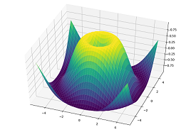
Axes3D

from matplotlib import cm
from mpl_toolkits.mplot3d import Axes3D

X = np.arange(-5, 5, 0.25)
Y = np.arange(-5, 5, 0.25)
X, Y = np.meshgrid(X, Y)
R = np.sqrt(X**2 + Y**2)
Z = np.sin(R)

fig = plt.figure()
ax = Axes3D(fig)
ax.plot_surface(X, Y, Z, rstride=1, cstride=1, cmap=cm.viridis)
plt.show()

Animation

import matplotlib.animation as animation

fig, ax = plt.subplots()
x = np.arange(0, 2*np.pi, 0.01)
line, = ax.plot(x, np.sin(x))
def init():  # only required for blitting to give a clean slate.
    line.set_ydata([np.nan] * len(x))
    return line,
def animate(i):
    line.set_ydata(np.sin(x + i / 100))  # update the data.
    return line,
ani = animation.FuncAnimation(
    fig, animate, init_func=init, interval=2, blit=True, save_count=50)
plt.show()